Time varying functions

While it is possible to construct arbitary time varying functions for use in summer2 models, there are a few cases that are sufficiently common for convenience functions to be supplied.

In particular, we cover the interpolation of sparse data points into their floating point equivalents (functions operating across the real numbers), as well as the composition of such functions into more complicated forms.

from summer2 import CompartmentalModel

# Import the Parameter and Time graphobject definitions
from summer2.parameters import Parameter, Time

# Convenience methods for time varying functions are contained in this module
from summer2.functions import time as stf

# ... and some external libraries
import numpy as np
import pandas as pd
from jax import numpy as jnp

Linear interpolation

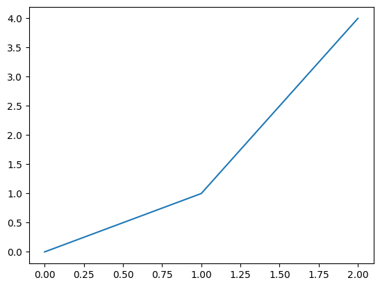
# Construct some synthetic data to interpolate

# x points (index)
x_points = np.array((0.0,1.0,2.0))
# y points (data)
y_points = x_points ** 2.0

s = pd.Series(index=x_points, data=y_points)
s.plot()

<Axes: >

# Interpolators are accessed via the get_*_interpolation_function functions

f_go = stf.get_linear_interpolation_function(x_points, y_points)
f_go

Function: 'interpolate_linear', args=(ModelVariable time, Function: 'ge...,), kwargs={}), Function: 'ge...,), kwargs={})), kwargs={})

# Although jax does not natively support Pandas datatypes, the interpolator constructors
# will recognise these as inputs and convert them appropriately, so it is often more
# convenient to use these values directly if your data is already in a Pandas Series

f_go = stf.get_linear_interpolation_function(s.index, s)
f_go

Function: 'interpolate_linear', args=(ModelVariable time, Function: 'ge...,), kwargs={}), Function: 'ge...,), kwargs={})), kwargs={})

Inspecting the graph

As with all ComputeGraph Functions, we can inspect the graph to determine the structure of the resulting object.

Our x and y inputs are captured as Data objects, which are then processed by the get_scale_data function; this simply processes the inputs in a way that is easier to consume by the internal functions of the final interpolator.

f_go.get_graph().draw()

While we could construct a callable directly from the graph, it is often quicker to use the get_time_callable convenience function, which will provide a callable taking a float or array as its time argument, and an optional parameters dictionary (we will cover this in the next section).

Note that the returned function is a compiled jax function, and as such will return jax.Array types as its output

ft = stf.get_time_callable(f_go)
ft(0.5)

Array(0.5, dtype=float64)

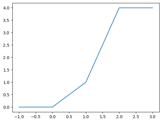
# To test the function across its whole domain, use an array as input

tvals = np.linspace(-1.0,3.0,101)
yvals = ft(tvals)

Visualising the resulting output shows that we capture the data as expected.

Outside the original bounds (x points), our function simply extends the first and last (y) values of the input

# Plot the results using Pandas
pd.Series(index=tvals,data=yvals).plot()

<Axes: >

Using GraphObjects as arguments

In the previous example, we have directly supplied numerical arrays as the inputs to our interpolator.

There will be many practical situations where the required inputs depend on runtime information, such as Parameters, or the outputs of other Functions, and the below examples detail such use cases

# Example 1 - fixed x (index) points, but parameterized y values

x_points = np.array((0.0, 5.0, 10.0))
# Use a list here rather than an array - see Note below for details
y_points = [0.0,Parameter("inflection_value"),0.0]

f_param = stf.get_linear_interpolation_function(x_points, y_points)

f_param_callable = stf.get_time_callable(f_param)
f_param_callable(np.linspace(0.0,10.0,11), {"inflection_value": 2.2})

Array([0.  , 0.44, 0.88, 1.32, 1.76, 2.2 , 1.76, 1.32, 0.88, 0.44, 0.  ],      dtype=float64)

# Output changes as expected for parameterized input
stf.get_time_callable(f_param)(np.linspace(0.0,10.0,11), {"inflection_value": -0.1})

Array([ 0.  , -0.02, -0.04, -0.06, -0.08, -0.1 , -0.08, -0.06, -0.04,
       -0.02,  0.  ], dtype=float64)

Note: Attempting to construct an array directly from GraphObjects, as in the following code, will result in an error if called with jnp.array, or silently construct a nonsense array if using np.array

During model construction, our real intent is to construct a GraphObject that returns an array, rather than an Array that contains GraphObjects

jnp.array([Parameter('x'), 1.0])

TypeError: Value 'Parameter x' with dtype object is not a valid JAX array type. Only arrays of numeric types are supported by JAX.

The get_*_interpolation_function constructors will automatically handle a variety of input types - in the case of the list constructor, it will call summer2.functions.util.capture_array behind the scenes, which will build the appropriate array-returning GraphObject; see the graph output below

For this reason, always use the idiomatic list type as shown above, or for more complex types, construct an appropriate ComputeGraph Function to use as input to the interpolators.

f_param.get_graph().draw()

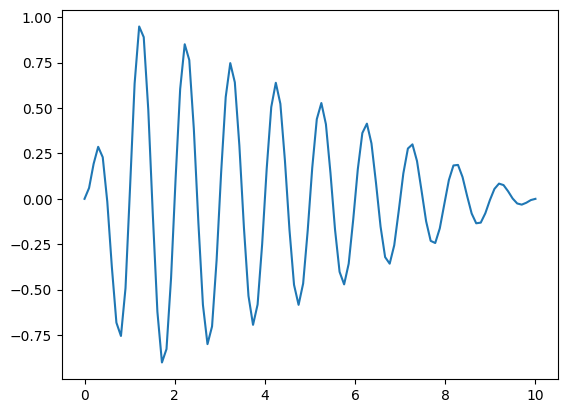
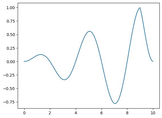
In the following example, we construct a complicated (but fairly arbitrary) Function, that produces a sinusoid with a user adjustable frequency, that scales to 0.0 at either end of the input domain (with a user specified inflection point ). Such functions might show up, for example, when modelling seasonably variable effects.

# Input contains GraphObjects - use a list
x_points = [0.0, Parameter("inflection_time"), 10.0]

# Calling numpy ufuncs on a GraphObject will produce another GraphObject
# It is of course possible to construct an equivalent Function manually,
# but much much easier to use the ufunc idiom for convenience
# Just remember that all internal model functions need to use jax,
# and so you must use jnp (rather than np) when writing your own functions
sin_t = np.sin(Time * Parameter("time_scale") * np.pi)

# Input contains GraphObjects - use a list
y_points = [0.0,sin_t,0.0]

f_complicated = stf.get_linear_interpolation_function(x_points, y_points)

f_complicated_callable = stf.get_time_callable(f_complicated)

in_domain = np.linspace(0.0,10.0,100)

# This function requires values for the Parameters we specified above
output = f_complicated_callable(in_domain, {"inflection_time": 1.0, "time_scale": 2.0})
pd.Series(output, index=in_domain).plot()

<Axes: >

output = f_complicated_callable(in_domain, {"inflection_time": 9.0, "time_scale": 0.5})
pd.Series(output, index=in_domain).plot()

<Axes: >

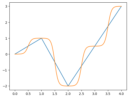
Sigmoidal Interpolators

Summer2 also provides a piecewise sigmoidal interpolator, available via the get_sigmoidal_interpolation_function

This takes an optional curvature argument, but has otherwise the same interface as the linear equivalent

This function produces output with a continuous derivative, so is useful for ‘smooth’ processes, or where extreme values might cause numerical noise with linear interpolation. Unlike spline interpolation, each piecewise segment is guaranteed never to exceed the bounds of its input values

# x points (index)
x_points = jnp.arange(5)
# y points (data)
y_points = jnp.array([0.0,1.0,-2.0,0.5,3.0])

s = pd.Series(index=x_points, data=y_points)

f_sig = stf.get_sigmoidal_interpolation_function(s.index, s) # curvature defaults to 16.0

in_domain = np.linspace(0.0,4.0, 101)

s.plot()
pd.Series(stf.get_time_callable(f_sig)(in_domain), index=in_domain).plot()

<Axes: >

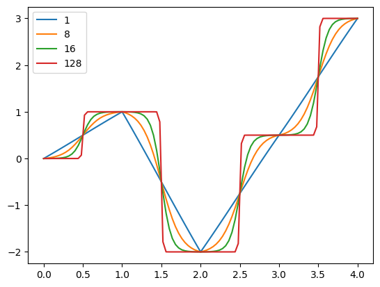
The curvature argument determines both the smoothness and the ‘squashing’ applied to each segment. At a value of 1.0, it is equiavalent to linear interpolation, and at high values it approximates a step function

in_domain = np.linspace(0.0,4.0, 101)

out_df = pd.DataFrame(index=in_domain)

for curvature in [1.0, 8.0, 16.0, 128.0]:
    f_sig = stf.get_sigmoidal_interpolation_function(s.index, s, curvature=curvature)
    out_df[curvature] = stf.get_time_callable(f_sig)(in_domain)

out_df.plot()

<Axes: >

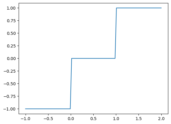
Piecewise functions

The interface to this function differs slightly from the interpolators shown above, in that the length of its x input (breakpoints) is always 1 less than that of the y input (values). This reflects the fact that its values are constant over ranges, rather than interpolated between known values at breakpoints

# Supply constant numerical arguments to produce a step function

f_step = stf.get_piecewise_function(np.array((0.0,1.0)), np.array((-1.0,0.0,1.0)))

in_domain = np.linspace(-1.0,2.0,101)
output = stf.get_time_callable(f_step)(in_domain)

pd.Series(output, index=in_domain).plot()

<Axes: >

Composition

get_piecewise_function is extremely useful for composing functions that might be expressed using if/else control structures in python, but would require the use of alternative techniques in jax

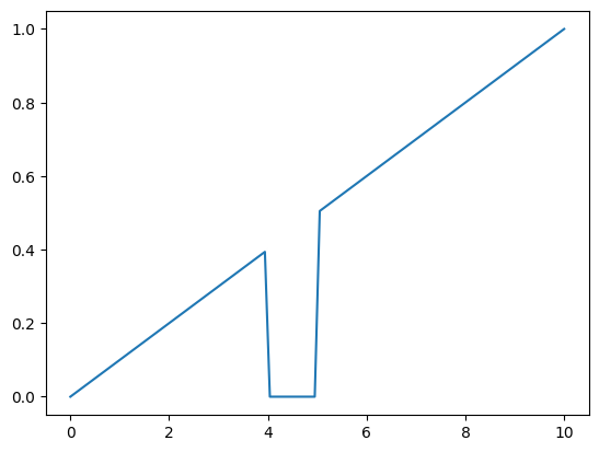
Consider the following example; the ‘baseline’ output is a linear ramp from 0.0 to 1.0, over the time domain of 0.0, 10.0

However, we also want to inject a fixed value of 0.0 between times 4.0 and 5.0 (perhaps we are modelling something like an intervention where no transmission should occur)

Typical python code for this may look something like the following;

def inject_zero(t):

    # Assume this function exists and does what we want it to...
    x = generate_linear_baseline(t)

    if 4.0 <= t < 5.0:
        return 0.0
    else:
        return x

# Create our 'baseline' linear interpolator
f_linear_baseline = stf.get_linear_interpolation_function(np.array((0.0,10.0)), np.array((0.0,1.0)))

# Use get_piecewise_function to compose the above function with the 0.0 range
f_overlay_zero = stf.get_piecewise_function(np.array((4.0,5.0)), [f_linear_baseline,0.0, f_linear_baseline])

in_domain = np.linspace(0.0,10.0,100)
output = stf.get_time_callable(f_overlay_zero)(in_domain)

pd.Series(output, index=in_domain).plot()

<Axes: >

While the above example only uses a single range (2 breakpoints), it can easily be extended to an arbitrary number of ranges, each with their own inputs

Using the functions in a CompartmentalModel

While all the above examples demonstrate how to evaluate time varying functions in a standalone context (which is valuable during development and debugging), you probably want to use them in a model!

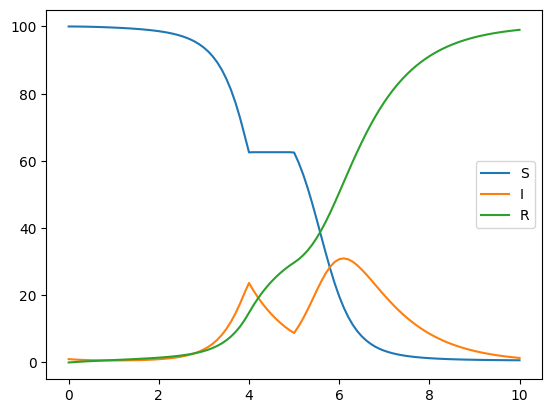
In this example we use the above ‘composed’ function to vary infection rates in a simple SIR model

m = CompartmentalModel([0.0, 10.0], ["S","I","R"], ["I"], timestep=0.1)
m.set_initial_population({"S": 100.0, "I": 1.0})

# Add an infection frequency flow that uses the time varying function defined above
m.add_infection_frequency_flow("infection", f_overlay_zero * Parameter("contact_rate"), "S", "I")

# Add a fixed rate recovery flow
m.add_transition_flow("recovery", 1.0, "I", "R")

# As expected, transmission gradually increases over time, but there is no transmission from times 4.0 to 5.0

m.run({"contact_rate": 10.0})
m.get_outputs_df().plot()

<Axes: >